Class 12 • Chapter 3

Current Electricity

The study of electric charges in motion. From thermal random drift to directed steady currents—master Ohm's law, Kirchhoff's circuit rules, and high-precision bridge networks.

I = n A e vd
Electric Current & Drift Velocity
The Life Analogy: Inside a conductor, billions of electrons wander randomly at blinding speeds, yet achieve zero net progress. Only when an external electric field gives them a shared direction do they 'drift' forward together to light up the world. Random effort is noise; directed persistence is power.

"Energy without direction is mere thermal chaos. Give your mind an electric field."

— The Physics of Purpose

"Resistance is not the enemy of current; it is the very reason the filament produces light."

— Law of Illumination

"Even the smallest drift velocity, sustained over time, creates an unstoppable surge."

— Principles of Drift

"In balanced circuits, no current is wasted. In a balanced mind, no energy is lost."

— Wheatstone Equilibrium

"What enters a junction must leave it. Every action, every thought preserves its consequence."

— Kirchhoff's Law of Life

"To endure the cold night alone under the moon is to prepare for the dawn of mastery."

— The Student's Solitude

Current Electricity Essentials

NCERT Core Definitions & Key Physical Facts

01

Electric Current (I)

The net rate of flow of electric charges crossing through a given cross-sectional area per unit time.

Mathematical Formulation: I = Q / t  |  I = dq / dt

SI Unit: Ampere (A) = Coulomb per second (C/s)

Scalar Nature: Although current possesses direction, it follows the rules of scalar addition, not vector algebra.
02

Ohm's Law

The steady current traversing a metallic conductor is directly proportional to the potential difference maintained across its terminals, provided physical parameters like temperature and strain remain constant.

Linear Relation: V ∝ I  &implies;  V = I · R

Condition for Validity: Applies strictly to linear ohmic conductors under steady thermal equilibrium.

03

Resistance (R)

The intrinsic opposition offered by the lattice ions of a conductor to the directed motion of drifting charge carriers.

Formula: R = V / I = ρ · (l / A)

SI Unit: Ohm (Ω) = Volt / Ampere (V/A)

Dependencies: Scales directly with conductor length (l), inversely with cross-section (A), and changes with temperature.

04

Resistivity / Specific Resistance (ρ)

A microscopic material property that measures how strongly a substance resists the passage of electric current, independent of geometric dimensions.

Relation: ρ = (R · A) / l = m / (n · e2 · τ)

SI Unit: Ohm-meter (Ω·m)

Characteristics: Dependent solely on the material's nature and ambient temperature.

05

Conductance (G)

The reciprocal of electrical resistance, measuring the degree of ease with which electric charge flows through a conductive medium.

Formula: G = 1 / R = I / V

SI Unit: Siemens (S) or mho (Ω-1)

06

Drift Velocity (vd)

The tiny net average velocity acquired by conduction electrons opposite to an externally applied electric field inside a conductor.

Expression: vd = - (e · E · τ) / m

Order of Magnitude: Typically tiny (~ 10-4 m/s), in contrast to random thermal speeds (~ 105 m/s).

SI Unit: Meter per second (m/s)

07

Electron Collision & Relaxation Time (τ)

Interactions where accelerated free electrons collide with oscillating positive lattice ions, dissipating directed kinetic energy as heat.

Relaxation Period (τ): The average time elapsed between two successive electron collisions.

Thermal Role: As temperature climbs, ion vibration widens, reducing τ and increasing electrical resistance.

08

Mobility (μ)

The magnitude of drift velocity acquired by a charge carrier per unit applied electric field strength.

Formula: μ = |vd| / E = (e · τ) / m

SI Unit: m2 / (V·s) or m2 · V-1 · s-1

Significance: A positive scalar index tracking charge carrier mobility.

09

Current Density (J)

A microscopic vector quantity defined as the electric current passing per unit cross-sectional area held normal to the charge flow direction.

Vector Form: I = ∫ J · dA  |  J = n · e · vd = σ · E

SI Unit: Ampere per square meter (A/m2)

Direction: Aligned with the local electric field vector E.

10

Electric Potential (V)

The external work required to bring a unit positive test charge from infinity to an electrostatic point without acceleration.

Relation: V = W / q

SI Unit: Volt (V) = Joule per Coulomb (J/C)

Circuit Role: Supplies the electric pressure gradient driving charges across closed paths.

11

Temperature Dependence of Resistance

Raising temperature amplifies ion lattice vibration, elevating collision frequency and reducing relaxation time (τ). For pure metallic conductors, this drives resistance upwards.

Thermal Formula: RT = R0 [ 1 + α (T - T0) ]

Temperature Coefficient (α): Positive for pure metals; negative for semiconductors and electrolytes where carrier density spikes with heat.

High-Yield Points

Critical Physics Facts

01

Scope of Ohm's Law

Ohm's Law is empirical rather than universal. It holds exclusively for linear conductors where resistance remains independent over applied potential ranges, failing in semiconductors, vacuum tubes, and electrolyte systems.

02

Determinants of Carrier Mobility

Mobility (μ) is influenced by temperature changes, material lattice impurities, crystal dislocations, and high electric field conditions.

03

Drift Velocity vs. Thermal Speed

Electrons undergo fast random thermal motion (~ 105 m/s) with zero net vector displacement. Superimposed on this is a slow directional drift velocity (~ 10-4 m/s), which establishes the net current.

04

Nature of Charge Carriers

In metallic wires, electric charge is carried entirely by negative conduction electrons moving through a fixed framework of positive ionic cores.

05

Mobility Impact on Current Output

Higher charge carrier mobility accelerates drift speed for a given electric field (vd = μ·E), producing larger current flow through identical cross-sections.

06

Operational Scope of Resistors

Resistors serve as fundamental passive components that provide calibrated impedance, regulating net electron passage and setting defined potential drops across circuit segments.

07

Thermal Inversion in Semiconductors

In intrinsic semiconductors, electrical resistance decreases with increasing temperature due to the rapid thermal generation of additional mobile electron-hole pairs, which dominates over ionic lattice scattering.

08

Inherent Nature of Resistivity

Specific resistance is an intensive physical property dependent entirely on the intrinsic lattice structure, atomic charge relaxation periods, and thermal agitation rather than specimen geometry.

Mathematical Architecture

Core Governing Relations

01

Rate of Charge Transport

I = dq / dt
Isteady = Q / t
IElectric Current (A)
dqDifferential Charge (C)
dtTime Interval (s)
02

Ohm's Macroscopic Law

V = I · R
I = V / R
VPotential Gradient (V)
IConduction Current (A)
RCircuit Resistance (Ω)
03

Geometric Scaling of Resistance

R = ρ · (l / A)
ρ = (R · A) / l
ρMaterial Resistivity (Ω·m)
lLength of Conductor (m)
ACross-Sectional Area (m2)
04

Charge Transport Mechanism

I = n · A · e · vd
J = n · e · vd
nCarrier Concentration (m-3)
eElementary Charge (1.6 × 10⁻¹⁹ C)
vdMean Drift Velocity (m/s)
05

Drift Kinematics Under Field

vd = - (e · E / m) τ
|vd| = (e · E · τ) / m
EApplied Field Vector (V/m)
mRest Mass of Electron (kg)
τMean Collision Relaxation Time (s)
06

Microscopic Current Density

J = I / A = σ · E
J = (n · e2 · τ / m) E
JCurrent Density (A/m2)
σConductivity Matrix (S/m)
EElectric Field Intensity (V/m)
07

Specific Electrical Conductivity

σ = J / E = (n · e2 · τ) / m
σ = 1 / ρ
σConductivity (S/m)
nMobile Carrier Density (m-3)
τLattice Relaxation Window (s)
08

Carrier Drift Mobility Index

μ = |vd| / E
μ = (e · τ) / m
μMobility Factor (m2 · V-1 · s-1)
vdDrift Speed Magnitude (m/s)
EElectric Gradient (V/m)
09

Microscopic Derivation of Resistivity

ρ = 1 / σ = m / (n · e2 · τ)
R = m · l / (n · e2 · τ · A)
ρResistivity Constant (Ω·m)
mInertial Electron Mass (kg)
nCarrier Density (m-3)
10

Thermal Dynamics of Resistivity

ρT = ρ0 [ 1 + α (T - T0) ]
RT = R0 [ 1 + α (T - T0) ]
ρTResistivity at Operating Temperature T (Ω·m)
ρ0Base Resistivity at Standard Temperature T0 (Ω·m)
αThermal Resistance Coefficient (K-1)
T - T0Thermal Increment (ΔT in K or °C)
Ohm's Law Exceptions

Limitations of Ohm's Law

Detailed breakdown of why certain materials and electronic devices deviate from standard V-I linearity.

CONDITION 01

Non-Proportionality of Voltage and Current

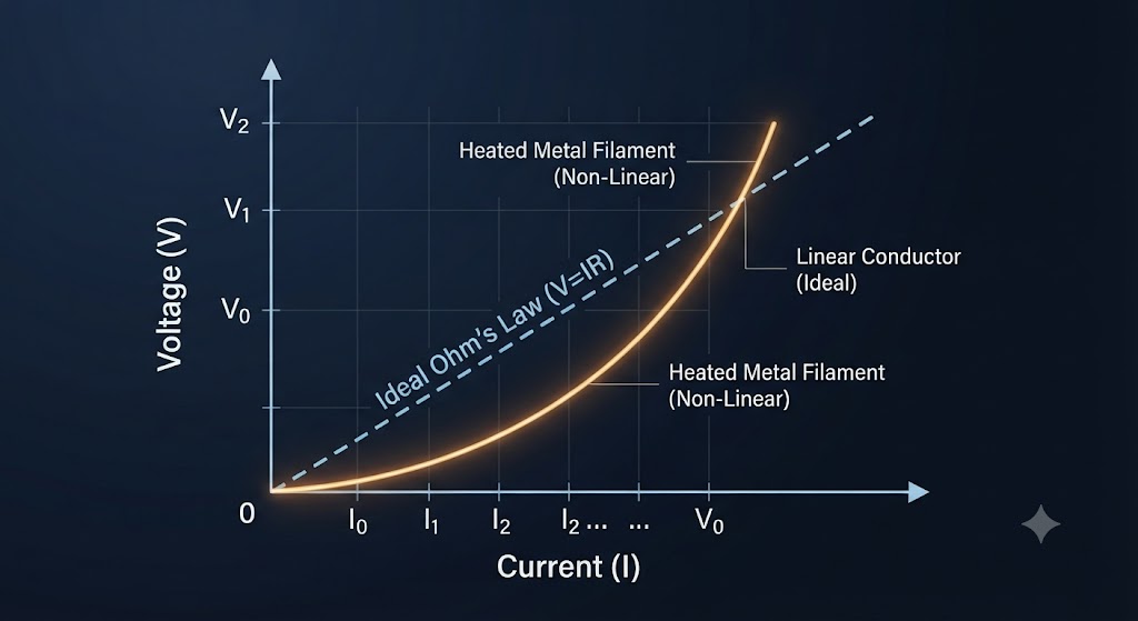
Ohm's Law states that voltage is directly proportional to current (V ∝ I), which produces a straight-line graph. However, in real metallic conductors (such as a heated lamp filament), heavy current causes internal Joule heating.

Physics Mechanism:

When a conductor gets hot, metal atoms vibrate violently, increasing electron collisions. This shortens the relaxation time (τ) and raises the resistance. Because resistance is no longer constant, the V-I graph bends upward away from the straight line.

Mathematical View: R = dV / dI ≠ Constant
V-I Curve for Non-Ohmic Conductor (Heated Filament)
Non-Linear V-I Characteristic Curve
Verified Educational Graphic • Shorveer Notes
CONDITION 02

Directional Dependence of Current (Rectification)

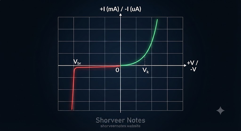
Ohm's law assumes that reversing the battery polarity should give an equal current magnitude in the opposite direction. Semiconductor electronic devices completely break this rule.

Physics Mechanism:

In p-n junction diodes, forward bias voltage lowers the internal barrier, allowing large milliampere (mA) currents to flow. Conversely, reverse bias widens the barrier, restricting flow to tiny microampere (μA) leakage currents.

Mathematical View: I(Forward) >> I(Reverse) for same |V|
V-I Characteristics of a P-N Junction Diode
Diode V-I Characteristic Graph
Verified Educational Graphic • Shorveer Notes
CONDITION 03

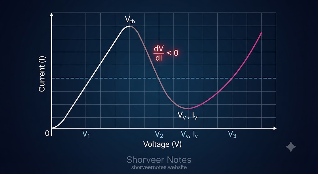
Non-Unique V-I Relationship & Negative Resistance

Normally, a single voltage value corresponds to a single current value. Advanced compound semiconductors break this rule, allowing multiple distinct voltage values to produce the exact same current level.

Gunn Effect & Valley Transfer Mechanics:

In Gallium Arsenide (GaAs), strong electric fields transfer conduction electrons into a higher energy valley where their effective mass increases, reducing drift velocity. This drop in current with increasing voltage creates a zone of Negative Differential Resistance (dV/dI < 0), widely used in microwave oscillators.

Differential Criterion: Rdiff = dV / dI < 0   (Negative Slope Zone)
Multi-Valued V-I Curve & Negative Differential Resistance (GaAs)
Gunn Diode Negative Resistance Characteristic
Verified Educational Graphic • Shorveer Notes
Current Electricity • Chapter 3

Temperature Dependence of Resistivity

Comprehensive analysis of how electrical resistivity (ρ) varies with absolute temperature (T) across metals, alloys, and semiconductors.

Core Mathematical Approximations & Notations

The electrical resistivity of a material changes with temperature and can be mathematically approximated using linear temperature coefficients.

Equation 01
ρT = ρ0 [1 + α(T - T0)]

Linear relation for temperature dependence of resistivity.

Equation 02
ρ = m / (n e2 τ)

Microscopic expression based on free electrons and relaxation time.

Nomenclature & Standard Notations:

  • ρT: Resistivity of the material at target absolute temperature T.
  • ρ0: Reference resistivity at initial standard temperature T0.
  • α: Temperature coefficient of electrical resistivity (positive for metals, negative for semiconductors).
  • m: Mass of a free electron ($9.1 \times 10^{-31}\text{ kg}$).
  • n: Number density of free electrons (free electrons per unit volume).
  • e: Elementary charge of an electron ($1.6 \times 10^{-19}\text{ C}$).
  • τ: Average relaxation time between consecutive electronic collisions.
METALS & ALLOYS

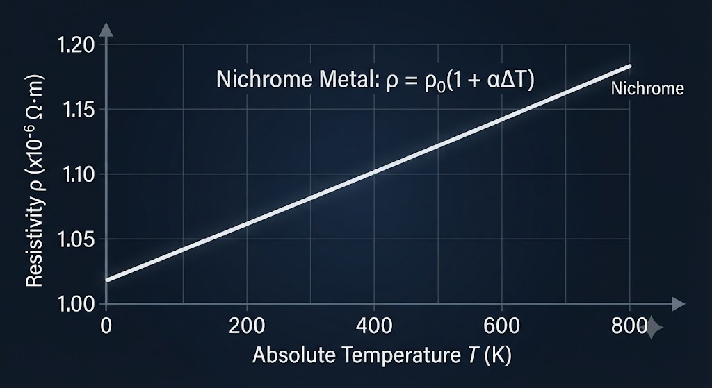
Behavior of Metals & Alloys (e.g., Nichrome, Manganin)

In metals, the free electron density (n) remains largely unaffected by temperature changes. However, higher temperature increases thermal agitation, causing frequent atomic collisions which drastically reduce relaxation time (τ).

Key Takeaways:

As temperature rises, resistance and resistivity (ρ) increase almost linearly. Alloys like Nichrome, Manganin, and Constantan show weak temperature dependence with high baseline resistivity, making them ideal for standard wire-wound resistors. For metals, temperature coefficient (α) is positive.

Figure: Resistivity ρ of Nichrome as a function of Absolute Temperature T
Nichrome Metal Resistivity Temperature Graph
Verified Educational Graphic • Shorveer Notes
SEMICONDUCTORS

Behavior of Semiconductors & Insulators

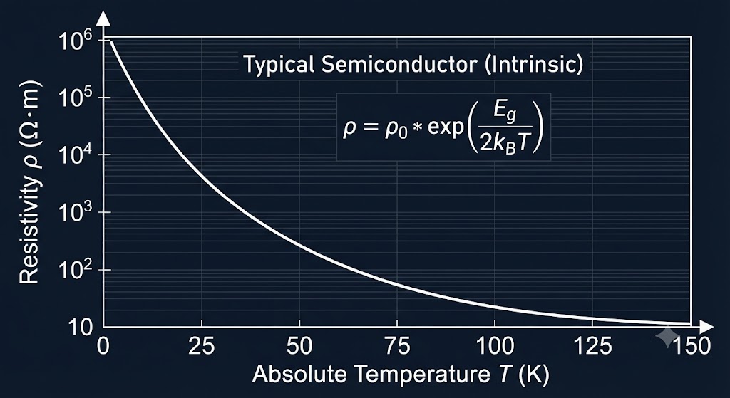
Unlike metals, semiconductors (such as Silicon and Germanium) and insulators exhibit a completely opposite trend. Their resistivity drops exponentially as temperature increases.

Mechanism & Band Gap:

In semiconductors, the charge carrier density (n) increases exponentially with temperature due to thermal excitation across the band gap. This rapid increase in free carriers overrides any reduction in relaxation time, causing resistivity (ρ) to fall sharply. They possess a negative temperature coefficient (α < 0).

Figure: Temperature Dependence of Resistivity for a Typical Semiconductor
Semiconductor Resistivity Exponential Decrease Graph
Verified Educational Graphic • Shorveer Notes
Fundamental Properties • Chapter 3

Material Classifications & Fundamental Properties

Detailed comparative analysis of conductors, insulators, along with a rigorous distinction between electrical resistance and resistivity.

1. Comparative Breakdown: Conductors vs. Insulators

CONDUCTORS

Electrical Conductors

Materials that permit the unhindered flow of electric charges due to an abundance of free conduction electrons.

  • Charge Mobility: Allow the free and rapid flow of electric charges.
  • Resistance Level: Possess exceptionally low electrical resistance to current flow.
  • Electron Binding: Valence electrons are loosely bound to parent nuclei and move easily through the lattice.
  • Practical Applications: Extensively utilized for electrical wiring, transmission lines, connector pins, and active circuit components.
  • Standard Examples: Copper (Cu), Aluminum (Al), Silver (Ag).
INSULATORS

Electrical Insulators (Dielectrics)

Materials that restrict the free movement of electric charges, preventing current flow under normal operating conditions.

  • Charge Mobility: Do not allow the free flow of electric charges.
  • Resistance Level: Possess extremely high electrical resistance.
  • Electron Binding: Valence electrons are tightly bound by covalent or ionic bonds and do not move freely.
  • Practical Applications: Deployed for electrical insulation, sheathing, protective barriers, and safety housings.
  • Standard Examples: Rubber, Glass, Ebonite, Plastic.

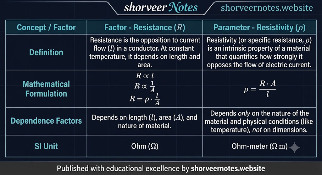
2. Fundamental Distinction: Resistance vs. Resistivity

Parameter / Feature Electrical Resistance (R) Electrical Resistivity (ρ)
Definition & Nature The inherent property of a specific physical component or object that obstructs current flow. An intrinsic characteristic property belonging to the material itself, independent of dimensions.
SI Unit of Measurement Measured in Ohms (Ω). Measured in Ohm-meters (Ω·m).
Dependency on Dimensions Directly depends on physical geometry (length l and cross-sectional area A). Completely independent of physical dimensions (length or cross-sectional area).
Material Consistency Can vary across different samples and shapes of the exact same substance. Remains strictly constant for any given material at a fixed temperature.
Core Functional Role Determines the exact total opposition offered by a device or component to current. Determines the fundamental material-level opposition to electric current per unit geometry.
Electrical Instruments • Chapter 3

Ammeter vs. Voltmeter Comparison

Detailed comparative breakdown of measuring instruments used for tracking electrical current and potential differences in circuits.

Parameter / Feature Ammeter Voltmeter
Primary Function Measures the electric current flowing through a specific branch or loop of a circuit. Measures the electric potential difference (voltage) across a component or resistor.
Circuit Connection Connected in series with the circuit so that the entire target current passes through it. Connected in parallel across the component whose voltage is being measured.
Internal Resistance Designed to have an exceptionally low resistance to prevent altering or restricting circuit current. Designed to have an extremely high resistance to minimize any current drawing through the meter.
SI Unit & Scale Measured in Amperes (A) or milliamperes (mA). Measured in Volts (V) or millivolts (mV).
Operational Utility Utilized to monitor, regulate, and control current levels safely within electronic systems. Utilized to measure voltage drops across components and test circuit integrity.
NCERT High-Yield Core Definitions • Chapter 3

Fundamental Electrical Definitions & Circuit Concepts

Comprehensive and expanded breakdown of essential physics definitions, commonly asked in 1-mark board queries and conceptual derivations.

CONCEPT 01

Electrical Energy

Electrical energy is the total work done or energy produced by the movement of electric charges through a conductor. It represents the capacity of an electric current to perform mechanical, thermal, or chemical work.

SI Unit: Joules (J) or Watt-hour (Wh)
CONCEPT 02

Electric Power

Power in an electrical circuit is defined as the rate at which electrical energy is transferred or dissipated by an electric current over time. It dictates how fast work is done in a circuit.

SI Unit / Formula: Watts (W)  |  P = VI = I²R
CONCEPT 03

Electromotive Force (EMF - ε)

The EMF of a cell is the maximum potential difference between its two terminals when no current is flowing through the external circuit (open circuit condition). It represents the non-electrostatic work done to drive unit positive charge around the complete loop.

SI Unit: Volts (V)
CONCEPT 04

Internal Resistance of a Cell (r)

Internal resistance is the opposition offered by the electrolyte and electrodes of a source of electrical power (such as a cell or battery) to the internal flow of electric current. It causes a potential drop when current is drawn.

Symbol & Unit: Symbol: r  |  Unit: Ohms (Ω)
CONCEPT 05

Potential Difference (V)

Potential difference is the difference in electric potential between two specified points in a circuit under closed-circuit conditions. It acts as the driving force that causes electric charges to flow continuously.

SI Unit: Volts (V)  |  V = ε - Ir

Circuit Configurations: Series vs. Parallel Paths

Series Circuit Configuration

A circuit arrangement in which components are connected end-to-end along a single continuous path, ensuring that the exact same electric current flows through each individual component.

Parallel Circuit Configuration

A circuit configuration in which components are connected across common nodes, providing multiple independent branches for current to divide, while the potential difference across each parallel branch remains identical.

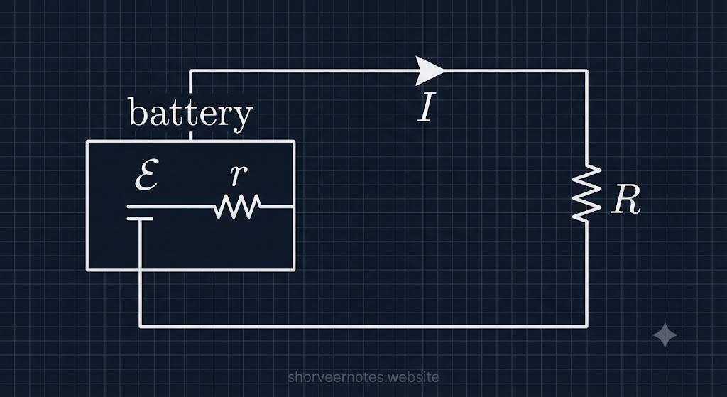
Figure: Cell with EMF (ε), Internal Resistance (r), and External Load (R)
Circuit Diagram showing EMF, internal resistance, and external load resistor
Verified Educational Graphic • Shorveer Notes
Chapter 3 • Core Concepts Summary

Important Facts: Cells & Batteries Revisited

Comprehensive and expanded breakdown of essential principles regarding electrical cells, their combinations, and energy dissipation.

FACT 01

Series Combination & Total Voltage

When identical electrical cells are connected in a series configuration, the positive terminal of one cell is linked to the negative terminal of the next. This arrangement **increases the total electromotive force (EMF)** of the combination, making it equivalent to the sum of the individual EMFs of all connected cells.

FACT 02

Parallel Combination & Current Capacity

In a parallel connection, all positive terminals are joined together, and all negative terminals are connected to a common node. While the overall EMF remains equal to that of a single cell, this configuration significantly **increases the total current capacity** (amperage) and discharge duration of the battery bank.

FACT 03

EMF Summation in Series Connection

For cells connected in series, the total EMF of the circuit is the simple arithmetic **sum of the EMFs** of each individual cell. In contrast, for cells connected in parallel, the total EMF of the battery system **remains the same** as the EMF of a single cell.

FACT 04

Total Internal Resistance Comparison

For cells connected in series, the total **internal resistance increases** (sum of individual resistances). In direct contrast, for identical cells connected in parallel, the total equivalent **internal resistance decreases** compared to the resistance of a single cell, allowing for higher current draw.

FACT 05

Definition of Electric Cells & Batteries

An electric cell is a fundamental device that converts stored **chemical energy into electrical energy**, thereby providing a potential difference to drive current in a circuit. A battery, in this context, is simply a practical collection or assembly of multiple individual electric cells connected together.

FACT 06

Cell Combinations & Practical Applications

Cell combinations are strategically utilized in a vast array of devices to meet specific power requirements. For instance, flashlights use cells in series to achieve higher voltage, while complex systems like electric vehicles and large UPS units employ sophisticated series-parallel combinations to attain both the desired voltage and immense current capacity for optimal performance.

FACT 07

Ohmic Power Loss (I²R Loss)

Ohmic loss, often termed **power loss or Joule heating**, is the unavoidable dissipation of electrical energy into heat as current flows through the inherent resistance (R) of any conductor, wire, or component within a circuit. This thermal energy conversion **reduces the overall electrical efficiency**, particularly in demanding high-power applications where significant currents generate substantial heat.

Current Electricity • Chapter 3

Fundamental Formulae: EMF, Power, & Cells

Comprehensive and expanded breakdown of essential electrical equations, including efficiency, power dissipation, and cell combinations.

1

Formula for Electrical Efficiency

η = (Useful energy output / Total energy input) × 100%

Defines the effectiveness of an electrical device in converting input energy to useful output energy.

2

Electric Power Dissipated in Circuit

P = I2R = V2/R = VI

Expresses the rate at which electrical energy is converted into heat (Joule heating) in a resistor.

P = Power (Watts, W) I = Current (Amperes, A) V = Voltage (Volts, V) R = Resistance (Ohms, Ω)
3

Definition of Electromotive Force (EMF - ε)

ε = Wext / q

EMF is the work done by non-electrostatic (external) forces per unit charge to move it around the complete circuit loop.

ε = EMF (Volts, V) Wext = Work done (Joules, J) q = Charge (Coulombs, C)
4

Terminal Voltage (V) Across a Cell

V = ε - Ir

Relates the terminal potential difference (V) of a cell to its EMF (ε), current (I), and internal resistance (r). It is less than EMF during discharge.

V = Terminal Voltage ε = EMF r = Internal Resistance
5

Current Flowing in Circuit with Internal Res.

I = ε / (R + r)

Ohm's law applied to a complete circuit loop, accounting for both external (R) and internal (r) resistances.

6

Two Cells in Series Combination

Equivalent EMF: εeq = ε1 + ε2
Equivalent Internal Resistance: req = r1 + r2

When cells are added in series, both their total EMF and total internal resistance add up linearly.

7

Two Cells in Parallel Combination

Equivalent EMF: εeq = (ε1r2 + ε2r1) / (r1 + r2)
Equivalent Internal Resistance: req = (r1r2) / (r1 + r2)

Parallel connection increases total current capacity while the combined EMF is determined by the weighted average of individual EMFs.

8

Generalized 'n' Parallel Cells

1/req = 1/r1 + 1/r2 + ... + 1/rn
εeq/req = ε1/r1 + ε2/r2 + ... + εn/rn

Formula for 'n' dissimilar cells connected in parallel using equivalent resistance method (similar to Kirchoff's approach).

Current Electricity • Chapter 3

Series vs. Parallel Combination of Resistors

Detailed comparative analysis of how current, voltage, resistance, power, and failure impact vary across series and parallel electrical networks.

Circuit Property Series Circuit Combination Parallel Circuit Combination
Electric Current (I) The same current flows through all individual components without any branching. The total current is the algebraic sum of currents flowing through individual parallel branches (Itotal = I1 + I2 + ... + In).
Potential Difference / Voltage (V) The total applied voltage is the sum of the potential drops across each separate component (Vtotal = V1 + V2 + ... + Vn). The same voltage is applied and shared equally across all individual parallel components or branches.
Equivalent Resistance (R) The total resistance is the direct arithmetic sum of individual resistances:
Rtotal = R1 + R2 + ... + Rn (Increases total value).
The reciprocal of total equivalent resistance is the sum of reciprocals of individual resistances:
1/Rtotal = 1/R1 + 1/R2 + ... + 1/Rn (Decreases total value, always less than the smallest individual resistor).
Power Distribution (P) Power dissipation varies directly with each component's resistance; higher resistance consumes more power (P = I2R). Power can be distributed equally or inversely proportional to resistance; lower resistance branches consume higher power (P = V2/R).
Failure Impact & Reliability If one component fails or breaks, an open circuit is created, and the entire circuit stops working completely. If one component fails, the remaining parallel branches continue to function independently without interruption.
Practical Applications Utilized where a uniform current must pass through all elements in tandem, such as old-style decorative Christmas tree string lights. Employed in nearly all household electrical wiring and industrial systems where appliances operate independently at full line voltage.
Current Electricity • Chapter 3

Internal Resistance vs. External Resistance

Detailed comparative breakdown analyzing the fundamental differences between internal opposition within power sources and external circuit load resistance.

Comparative Feature Internal Resistance (r) External Resistance (R)
Core Definition The inherent opposition offered by the internal constituents (such as electrolytes and electrodes) of a power source to the flow of charge. The total opposition to current flow offered by the external network components, load devices, and wiring connected across the source terminals.
Physical Location Confined strictly within the boundaries of the power source itself (e.g., inside a battery cell or generator). Situated entirely outside the power source within the external circuit loop and connected load devices.
Operational Impact Causes an internal potential drop ($Ir$), which reduces the available terminal voltage and limits the maximum output current under load conditions. Directly governs and regulates the magnitude of the main electric current flowing through the entire circuit loop ($I = \frac{\varepsilon}{R+r}$).
Method of Measurement Cannot be measured directly; determined indirectly by comparing open-circuit and closed-circuit terminal voltage differences. Can be measured directly using a standard ohmmeter or digital multimeter across component terminals.
Key Dependencies Depends on the nature of the source, electrolyte concentration, temperature, electrode surface area, and separation distance. Depends on the physical geometry (length and cross-sectional area), material resistivity, and operating temperature of the load components.
Practical Examples Chemical electrolyte and electrode resistance inside lead-acid batteries, dry cells, or internal generator winding coils. Standard carbon/wire-wound resistors, indicator lamps, electric motors, heating elements, and electronic appliances.
Current Electricity • Chapter 3

EMF & Terminal Voltage: Visual Analysis

Detailed graphical breakdown of terminal voltage equations and core differences between Electromotive Force and Terminal Voltage.

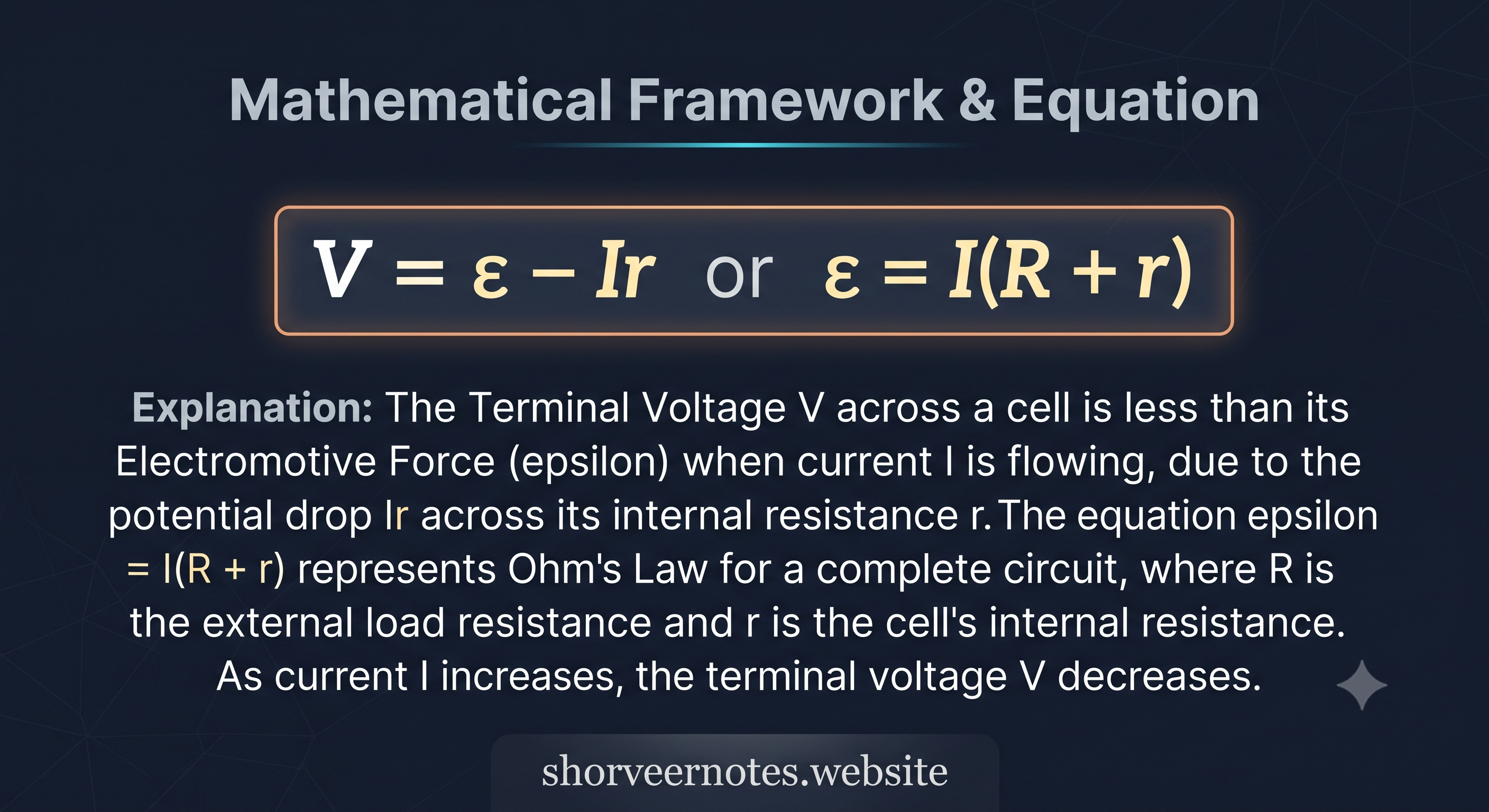
EQUATION 01

Mathematical Framework & Equation

Mathematical Framework and Equation V = epsilon - Ir

Shows how terminal voltage (V) drops below EMF (E) due to internal resistance potential loss (Ir)

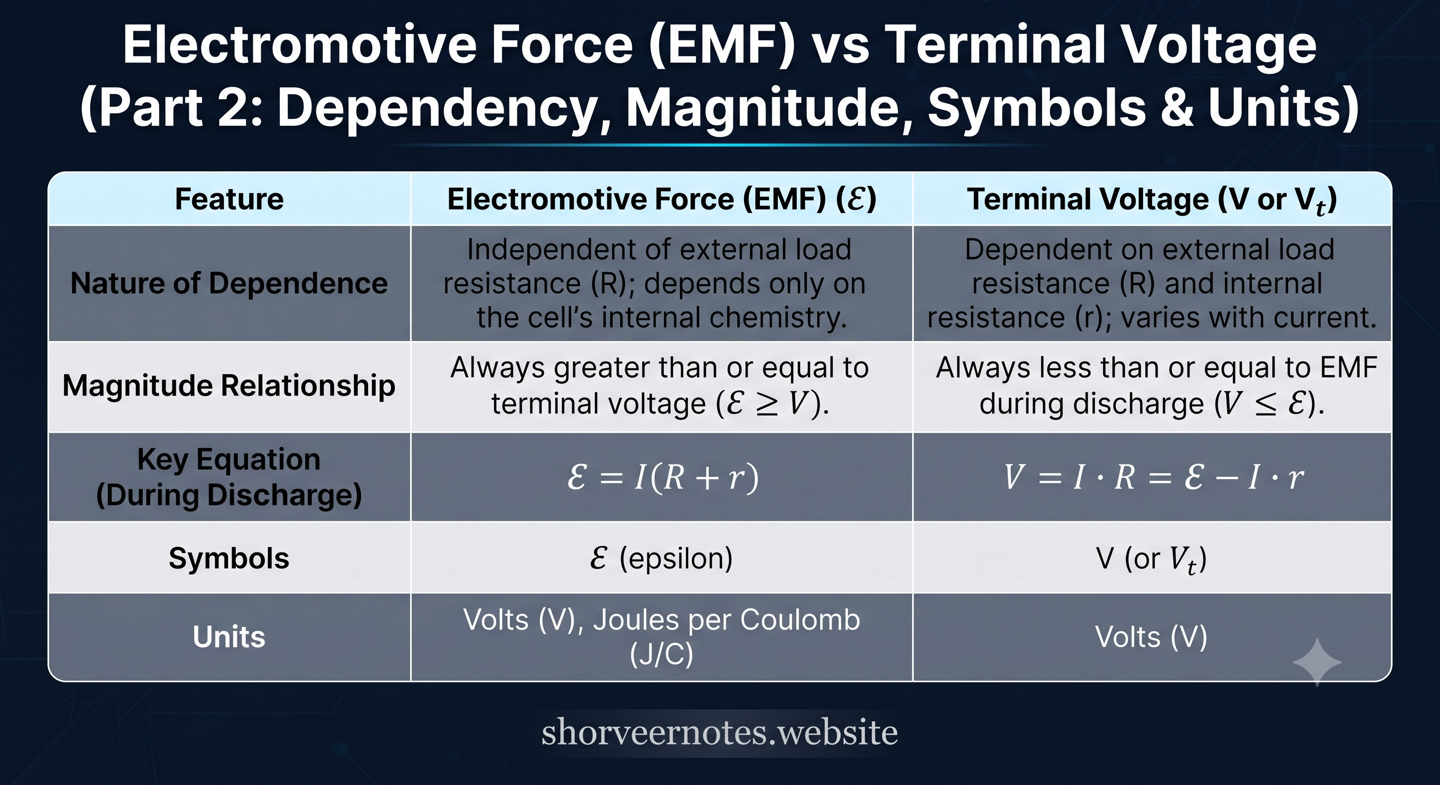
COMPARISON 02

EMF vs. Terminal Voltage Breakdown

Electromotive Force vs Terminal Voltage Comparison Table

Comprehensive comparative analysis highlighting dependency, magnitude relationships, key equations, and units.

Advanced Circuit Theorems & Analysis

Network Analysis: Kirchhoff's Laws & Wheatstone Bridge

Rigorous breakdown of electrical network terminologies, conservation laws, bridge balance conditions, and unknown resistance determination.

1. Essential Circuit Network Terminology

TERM 01

Electrical Node

A specific junction point or terminal in an electric circuit where two or more circuit components, conductors, or branches meet and connect together.

TERM 02

Closed Loop

A completely closed conducting path in a circuit network where no single node or component is encountered more than once during a full traversal.

TERM 03

Galvanometer

A highly sensitive electromechanical precision instrument utilized specifically to detect and quantify minute electric currents or null deflections in bridge circuits.

2. Fundamental Laws of Network Analysis

LAW I

Kirchhoff's First Rule (Junction Rule / KCL)

At any electrical junction or node, the algebraic sum of all electric currents meeting at that junction must be identically equal to zero ($\sum I = 0$).

Underlying Conservation Principle:

This rule is a direct mathematical consequence of the Law of Conservation of Charge. Total charge entering a node per unit time must equal the total charge leaving it, preventing any charge accumulation.

LAW II

Kirchhoff's Second Rule (Loop Rule / KVL)

Around any closed loop or mesh in an electrical network, the algebraic sum of all electrical potential differences (product of current and resistance) combined with sources of EMF must equal zero ($\sum \Delta V = 0$).

Underlying Conservation Principle:

This rule stems directly from the Law of Conservation of Energy, establishing that electrostatic force fields are conservative, meaning net potential change around a closed loop is zero.

3. Wheatstone Bridge & Precision Resistance Measurement

Structural Anatomy & Balanced Operating State

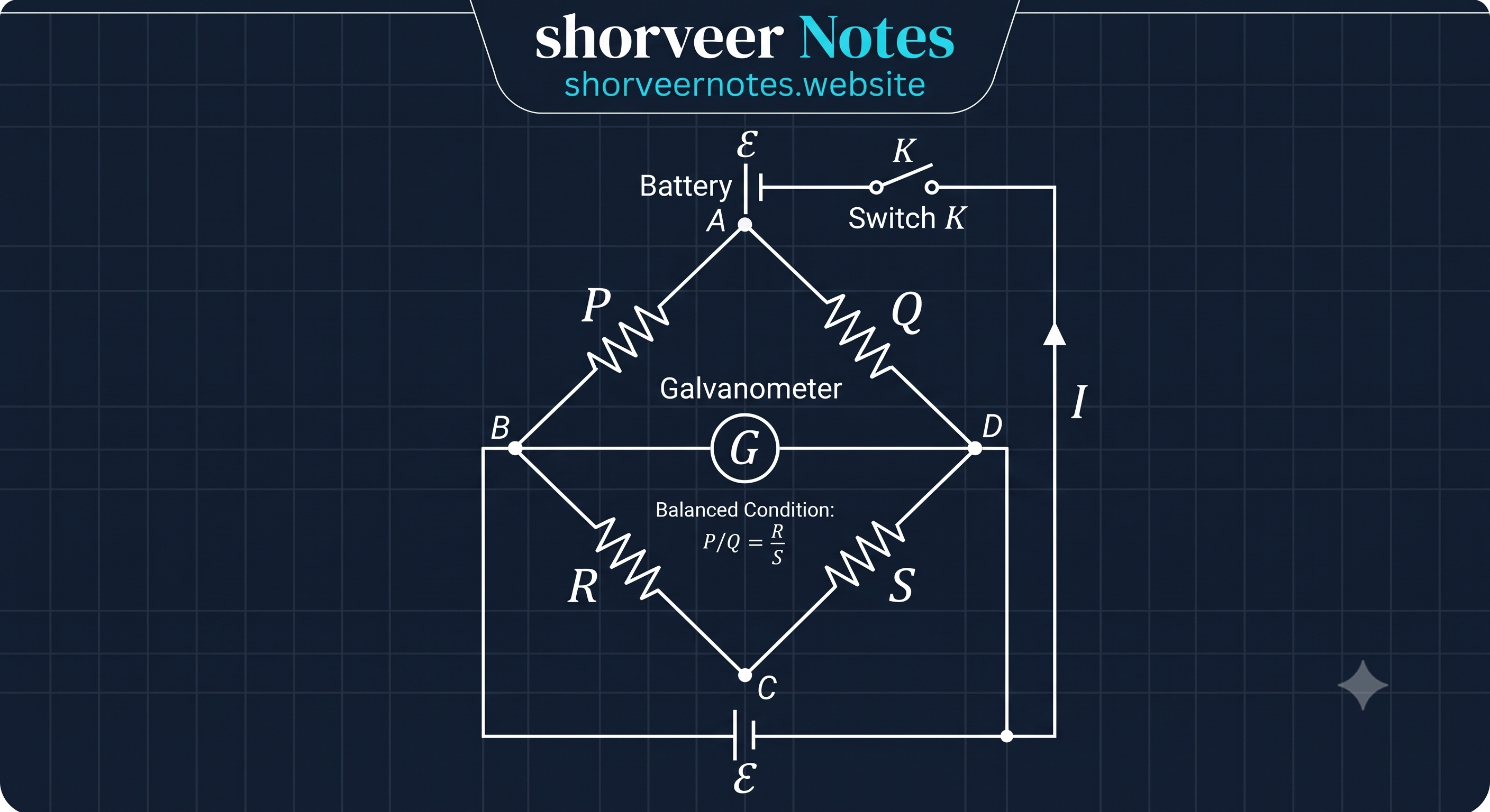
A Wheatstone Bridge is an ingenious bridge circuit comprising four distinct resistive arms arranged in a diamond configuration, powered by an external DC voltage source ($\text{E}$) with a sensitive galvanometer bridged across opposite junctions.

The Balanced Bridge Condition:

When the bridge is adjusted such that zero current flows through the galvanometer ($I_g = 0$), the bridge is termed balanced. Under this pristine condition, the potential at node $b$ equals node $d$, yielding the fundamental bridge ratio equation:

Balance Ratio: P / Q = R / S   ∴   Unknown S = Q × (R / P)
Figure: Standard Wheatstone Bridge Circuit Network
Wheatstone Bridge Circuit Network Diagram
Verified Educational Graphic • Shorveer Notes
High-Yield Conceptual Facts & Applications

Key Circuit Principles & Bridge Applications

Comprehensive breakdown of foundational laws, null measurement principles, and advanced industrial applications of bridge networks.

FACT 01

Applicability to DC & AC Circuits

Kirchhoff's rules are fundamental network laws that are not restricted solely to direct current (DC) systems. They apply universally to **both direct current (DC) and alternating current (AC) circuits**, provided that instantaneous values and phasor relationships are properly accounted for in time-varying networks.

FACT 02

KVL and Energy Conservation

Kirchhoff's Voltage Law (KVL / Second Rule) is fundamentally rooted in the **Law of Conservation of Energy**. It establishes that the total net work done in moving a unit positive charge around any complete closed conducting loop in an electrostatic field is identically zero.

FACT 03

KCL and Charge Conservation

Kirchhoff's Current Law (KCL / First Rule) is based strictly on the **Law of Conservation of Charge** within closed electrical networks. It enables engineers and physicists to systematically calculate unknown branch currents in complex multi-loop circuits where conventional series-parallel reductions fail.

FACT 04

Null Measurement Principle

The Wheatstone Bridge operates on the precision principle of **null measurement**, wherein the system is adjusted until zero current flows through the central galvanometer branch ($I_g = 0$). This zero-deflection state indicates precise electrical equilibrium and yields highly accurate, error-free resistance values.

FACT 05

Industrial & Scientific Applications (Strain Gauges)

Beyond laboratory resistance testing, the Wheatstone Bridge provides an exceptionally accurate method for measuring physical quantities in engineering. By incorporating **strain gauges** into its arms, tiny dimensional deformations can be translated into minute resistance shifts, allowing precise measurement of mechanical force, structural pressure, torque, and weight.

Core Circuit Theorems & Equations

Fundamental Laws & Bridge Balance Conditions

Comprehensive mathematical framework and analytical breakdowns of Kirchhoff's network rules and Wheatstone bridge equilibrium.

LAW 01

Kirchhoff's Voltage Law (Loop Rule - KVL)

∑around loop V = 0

The algebraic sum of all electric potential changes (voltage rises and voltage drops) encountered while traversing any closed loop in a circuit network is identically zero.

Physical Significance:

Based on the Law of Conservation of Energy, this equation ensures that total energy supplied by sources in a closed mesh equals total energy dissipated across loads.

LAW 02

Kirchhoff's Current Law (Junction Rule - KCL)

∑into junction I = ∑out of junction I

At any point or node in an electric circuit, the total sum of electric currents flowing directly into the junction equals the total sum of currents flowing away from it.

Physical Significance:

Grounded on the Law of Conservation of Charge, it dictates that electric charge cannot accumulate indefinitely at a single circuit junction.

CONDITION 03

Condition for Wheatstone Bridge Equilibrium

R1 / R2 = R3 / R4

A Wheatstone bridge is balanced when the potential difference across the galvanometer branch becomes zero ($V_b = V_d$), resulting in null deflection. Under this state, the ratio of resistances in opposite arms is equal.

Nomenclature & Arm Layout:

Where R1, R2, R3, and R4 represent the discrete resistances distributed across the four arms of the diamond bridge network. This relationship allows precise determination of any unknown resistance value.

Visual Master Tables & Frameworks

Comparative Circuit Analysis Infographics

High-yield comparative visual tables designed for rapid revision of core circuit laws, bridge configurations, and electrical measurement instruments.

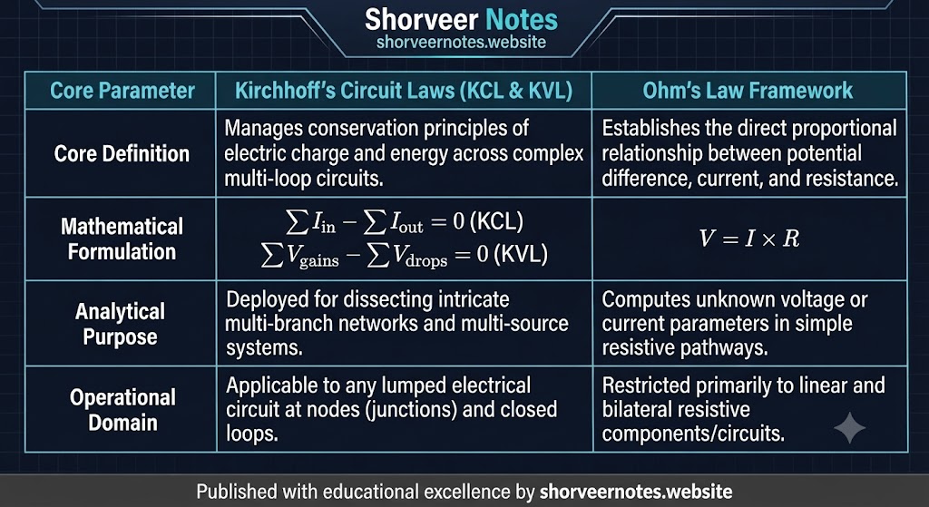
TABLE 01

Kirchhoff's Laws vs. Ohm's Law Framework

Kirchhoffs Circuit Laws vs Ohms Law Framework Comparison Table

Comparative breakdown of conservation principles, mathematical formulations, and operational domains across complex and simple resistive networks.

TABLE 02

Balanced vs. Unbalanced Wheatstone Bridge

Balanced vs Unbalanced Wheatstone Bridge Comparison Table

Detailed analysis of bridge operational states, ratio conditions, equipotential null points, and transducer utilities.

TABLE 03

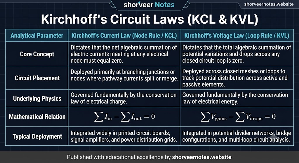
Kirchhoff's Circuit Laws (KCL & KVL) Deep Dive

Kirchhoffs Circuit Laws KCL and KVL Detailed Table

Comprehensive comparison of Node Rule (KCL) and Loop Rule (KVL), highlighting charge/energy conservation and mathematical equations.

TABLE 04

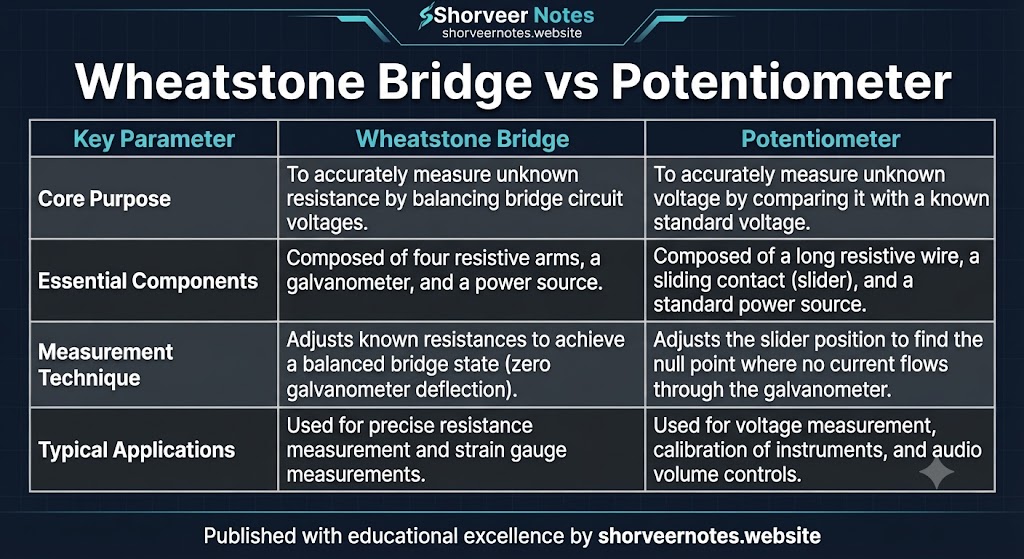
Wheatstone Bridge vs. Potentiometer

Wheatstone Bridge vs Potentiometer Comparison Table

Core technical contrast between measuring unknown resistances via bridge balance and precise voltage comparison via null deflection.

Master Visual Summaries & Frameworks

Comprehensive Circuit Analysis & Material Properties Infographics

High-yield visual reference tables and master summaries covering Ohm's law, resistance, conductance, network laws, and bridge instrumentation.

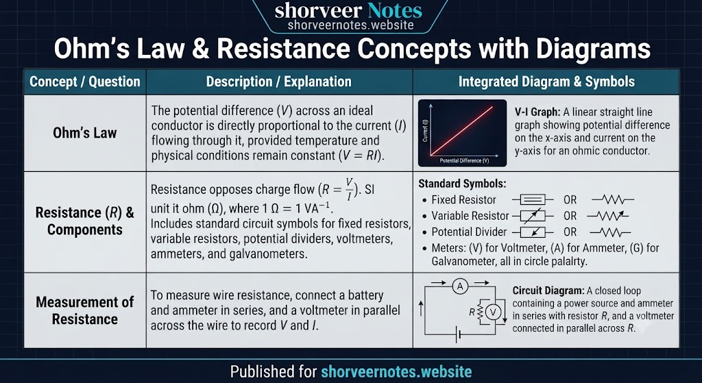
VISUAL 01

Ohm's Law, Resistance & Circuit Measurement

Ohms Law and Resistance Concepts with Diagrams

Visual guide outlining linear V-I characteristics for ohmic conductors, standard schematic circuit symbols, and standard ammeter-voltmeter connection setups.

VISUAL 02

Kirchhoff's Circuit Laws Master Table

Kirchhoffs Circuit Laws KCL and KVL Master Table

Structured comparative layout detailing node rules (KCL), loop rules (KVL), conservation laws, mathematical relations, and real-world system deployments.

VISUAL 03

Wheatstone Bridge vs. Potentiometer

Wheatstone Bridge vs Potentiometer Comparison Table

Technical comparison highlighting core operating purposes, internal bridge/wire components, null measurement techniques, and practical laboratory utilities.

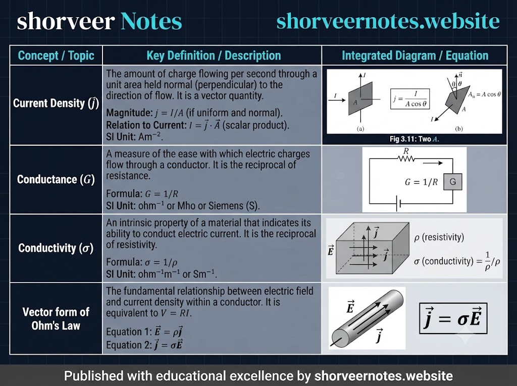
VISUAL 04

Current Density, Conductance & Conductivity

Current Density, Conductance, Conductivity and Vector Ohm Law

Microscopic and macroscopic framework illustrating current density vector formulations, material conductance, conductivity, and the vector form of Ohm's Law.

VISUAL 05

Resistance (R) vs. Resistivity (ρ) Master Breakdown

Resistance versus Resistivity Master Comparison Table

Definitive comparative matrix differentiating component opposition (resistance) from intrinsic material property (resistivity), complete with formulas and dimensional dependencies.

Microscopic Charge Dynamics & Derivation

Mechanism of Charge Flow, Drift Velocity & Relaxation Time

Comprehensive theoretical breakdown of free electron motion in metallic conductors under thermal agitation and external electric fields.

1. Electron Dynamics in the Absence of an Electric Field

Metallic conductors possess an immense abundance of free conduction electrons—approximately 1028 m-3 at room temperature. In the absence of any external electric field, these electrons are in a state of continuous, chaotic thermal motion.

Thermal Velocity

At room temperature, random thermal velocities of free electrons are extremely high, on the order of 105 m/s.

Isotropic Distribution

These velocities are distributed randomly in all directions with no preferred orientation, meaning electrons move equally in all paths.

Zero Net Flow

The vector average of all random thermal velocities across N electrons is identically zero: uavg = 0, resulting in zero net current.

2. Action of an External Electric Field & Acceleration

When an external electric field (E) is applied across the conductor, each free electron experiences an electrostatic force (F = -eE) directed opposite to the field due to its negative charge.

Acceleration (a) = Force / Mass = -eE / m

Where m represents the rest mass of an electron and a is the steady acceleration acquired between successive ionic collisions.

Inter-Collision Dynamics & Relaxation Time:

As electrons accelerate under the field, they frequently collide with vibrating positive metal ions or other lattice defects. Between two successive collisions, an electron gains a directional velocity component opposite to E. However, this accumulated velocity is randomized during the next collision, forcing the electron to start afresh with thermal velocity.

  • Relaxation Time (τ): The average time interval elapsing between two successive electronic collisions. For typical metals, it is on the order of 10-14 seconds.
  • Drift Velocity (vd): The small, steady average velocity acquired by free electrons in a direction opposite to the externally applied electric field.
    Final Equation: vd = -(eEτ) / m.
Microscopic Dynamics & Ohm's Law Framework

Relation Between Current, Drift Velocity & Microscopic Ohm's Law

Comprehensive mathematical derivation connecting macroscopic current with microscopic electron drift, resistivity, and vector field formulations.

1. Relation Between Electric Current and Drift Velocity

Consider a conductor of length l, uniform cross-sectional area A, across which a potential difference V is applied. The electric field E set up inside is given by E = V / l.

Electron Density (n)

Number of free electrons per unit volume of the conductor.

Total Charge (q)

Total volume = A · l, total electrons = n A l, hence total charge q = e n A l.

Current Derivation (I)

Time taken to cross length l is t = l / vd. Therefore, current I = q / t = e n A vd.

Current Formula: I = n e A vd   |   Current Density Vector: j = n e vd

Relates macroscopic electric current directly with the microscopic drift velocity of free charge carriers.

2. Microscopic Deduction of Ohm's Law

We substitute the expression of drift velocity vd = (e E τ) / m (where E = V / l) into the current equation:

I = n e A [ (e V τ) / (m l) ] = (n e2 A τ V) / (m l)

Rearranging terms to find the ratio of potential difference to current (V / I):

V / I = (m l) / (n e2 τ A) = Constant (R)

Since m, l, n, e, τ, and A remain constant at a fixed temperature, V / I yields a constant resistance R = (m l) / (n e2 τ A), thereby successfully proving Ohm's Law.

3. Resistivity and Vector Form of Ohm's Law

Resistivity in Terms of Relaxation Time:

Comparing R = ρ(l / A) with our derived resistance formula R = (m l) / (n e2 τ A), we get the intrinsic resistivity equation:

ρ = m / (n e2 τ)

Notice that resistivity ρ is completely independent of the physical dimensions of the conductor and depends solely on electron density (n) and relaxation time (τ).

Vector Form of Ohm's Law (j = σ E):

Starting from current density j = n e vd and substituting vd = -(e E τ) / m:

j = n e [ -(e E τ) / m ] = [ (n e2 τ) / m ] E

Since conductivity σ = 1 / ρ = (n e2 τ) / m, we arrive at the definitive vector formulation:

j = σ E   or   E = ρ j
Microscopic Origin & Factors of Resistance

What Causes Resistance in a Conductor?

Comprehensive breakdown explaining how atomic collisions, relaxation time, and physical dimensions govern electrical resistance.

1. The Fundamental Cause: Atomic Collisions

Collisions are the basic cause of electrical resistance. When a potential difference is applied across a conductor, its free electrons get accelerated. On their way through the lattice, they frequently collide with vibrating positive metal ions.

Resistivity Relation: ρ = m / (n e2 τ)

Larger the number of collisions per second, smaller is the relaxation time (τ), and consequently larger will be the resistivity (ρ).

2. Factors Affecting Conductor Resistance

Nature of Material

The number of collisions that electrons make depends on the arrangement of atoms or ions in a conductor. Thus, resistance depends entirely on the nature of the material (e.g., copper, silver, aluminum).

Length of the Conductor

The resistance of a conductor depends directly on its length. A long wire offers more resistance than a short wire because there will be a greater number of cumulative collisions in a longer wire.

Cross-Sectional Area

Resistance depends inversely on the cross-sectional area. A thick wire offers less resistance than a thin wire because a thick wire provides more available area and pathways for the smooth flow of electrons.

Charge Carrier Dynamics & Conductivity

Mobility and Conductivity of Semiconductors

Comprehensive theoretical breakdown of carrier mobility, relations with electric current, and semiconductor conductivity formulations.

1. Concept of Mobility (μ)

The conductivity of any material is due to its mobile charge carriers. These may be free electrons in metals, positive and negative ions in electrolytes, and both electrons and holes in semiconductors.

Mobility Formula: μ = vd / E

The mobility of a charge carrier is defined as the magnitude of drift velocity acquired per unit electric field.

Derivation via Drift Velocity

Since vd = (q E τ) / m, substituting this gives mobility: μ = τ / m

Electrons vs Holes

For an electron: μe = (e τe) / me
For a hole: μh = (e τh) / mh

Units of Mobility

SI Unit: m2 V-1 s-1
Practical Unit: cm2 V-1 s-1 (1 m2V-1s-1 = 104 cm2V-1s-1)

2. Relation Between Current and Mobility

For a Metallic Conductor:

Electric current is given by I = enAvd. Substituting drift velocity vd = μeE yields the relation: I = enA μe E.

For a Semiconductor (Electrons and Holes):

Semiconductor conductivity depends on both electrons and holes. Total current is the sum of electron and hole currents:

I = Ie + Ih = enAμeE + epAμhE = eAE (nμe + pμh)

Where n and p represent the electron and hole concentrations (densities) in the semiconductor.

3. Total Conductivity (σ) of a Semiconductor

Equating the current expression derived from microscopic carrier motion with Ohm's macroscopic law relation (I = (EA) / ρ) yields the final conductivity formula:

σ = e (nμe + pμh)

This fundamental equation expresses the total electrical conductivity of a semiconductor in terms of carrier densities and mobilities.

Temperature Dependence & Material Behavior

Effect of Temperature on Resistivity & Temperature Coefficient

Comprehensive theoretical breakdown of how resistivity changes with temperature in metals, supported by exact mathematical formulations and vector-rendered graphs.

1. Temperature Dependence in Metals

The resistivity of any material depends on the number density (n) of free electrons and the mean collision time (τ) through the relation: ρ = m / (n e2 τ).

Mechanism in Metals

In metals, n is nearly independent of temperature. As temperature increases, thermal speed and ionic vibrations increase, causing more frequent collisions. Thus, mean collision time (τ) decreases, leading to an increase in resistivity (ρ).

Linear Temperature Variation

For most metals around and above room temperature, resistivity increases linearly. At any temperature T, it is given by: ρ = ρ0 [1 + α (T - T0)]

2. Formula Notations & English Meanings

ρ (Rho): Electrical Resistivity at temperature T (Ohm-meter, Ω·m)
ρ0 (Rho-zero): Resistivity at reference temperature T0 (usually 20°C)
α (Alpha): Temperature Coefficient of Resistivity (°C-1)
T & T0: Target Temperature and Reference Temperature (Kelvin or Celsius)
m: Mass of an electron
n: Free electron number density
e: Electronic charge
τ (Tau): Mean collision time / Relaxation time

3. Graphical Variations of Resistivity with Temperature

The graphical representation of resistivity variation for copper (non-linear at low temperatures) and nichrome (linear at high ranges):

(a) Copper: Low Temperature (Non-linear)

Temperature T (K) Resistivity (ρ) 0 50 100 150 0.2 0.4

At low temperatures, pure copper exhibits a non-linear higher power dependence of resistivity with temperature.

(b) Nichrome: High Temperature (Linear)

Temperature T (K) Resistivity (ρ) 0 200 400 600 800 1.00 1.10 1.20

Alloys like nichrome show a gradual, nearly linear increase in resistivity across wide temperature spans.

Alloys Behavior & Temperature Variation

Temperature Dependence of Resistance & Properties of Alloys

Detailed technical breakdown of how resistance varies with temperature in alloys like nichrome and manganin, complete with resistance-temperature formulations.

1. Temperature Dependence in Alloys (Nichrome & Manganin)

Alloys possess high intrinsic resistivity. However, alloys like nichrome exhibit a very weak temperature dependence, while manganin is almost completely independent of temperature changes.

Behavior at Absolute Zero

At absolute zero ($0\text{ K}$), a pure metal has negligibly small resistivity, whereas an alloy (like nichrome) retains some residual resistivity due to structural disorder.

Distinguishing Metals from Alloys

This distinct difference in residual resistivity at very low temperatures is a fundamental characteristic used experimentally to distinguish a pure metal from an alloy.

2. Resistance-Temperature Formula & Notations

Since resistance $R = \rho (l / A)$, it implies that $R \propto \rho$. Therefore, the temperature equation can be directly expressed in terms of resistances:

Rt = R0 (1 + α t)

Relates the resistance of a conductor at a given temperature rise.

Rt: Resistance of the conductor at target temperature t°C
R0: Reference resistance at 0°C baseline temperature
α (Alpha): Temperature coefficient of resistance (°C-1)
t: Rise in temperature above 0°C (°C)
Conductor Classifications & Circuit Limits

Ohmic vs. Non-Ohmic Conductors & Limitations of Ohm's Law

Comprehensive theoretical and graphical breakdown of materials obeying and deviating from Ohm's law, complete with V-I characteristics and SVG rendered graphs.

1. Limitations of Ohm's Law

Ohm's law is obeyed by many substances under certain specific conditions, but it is not a fundamental law of nature. There are many electrical devices and situations where the linear relationship between voltage and current breaks down.

2. Ohmic Conductors & Their V-I Characteristics

Conductors that strictly obey Ohm's law are called Ohmic conductors. For these, a linear relationship between voltage and current ($V \propto I$) holds good, and resistance ($R = V/I$) remains constant regardless of current magnitude.

(a) Pure Metal (Linear V-I)

+V -V +I -I O

Straight line passing through the origin for a metallic conductor under small currents.

(b) Electrolyte with Cu Electrodes

+V -V +I -I O

Linear V-I relationship for copper sulphate ($\text{CuSO}_4$) solution with copper electrodes.

3. Non-Ohmic Situations & Conductors

In non-ohmic scenarios, the resistance is not constant but current-dependent. Deviations typically manifest in four distinct types:

1. Non-Origin Pass

The straight line V-I graph does not pass through the origin.

2. Non-Linear Relation

The overall V-I relationship is non-linear (curved).

3. Sign Dependency

The V-I relationship depends on the sign of potential difference $V$ for the same absolute value of $V$.

4. Non-Unique Path

The V-I relationship is non-unique (multiple current values for a single voltage).

4. Metallic Conductor at Higher Currents (Thermal Deviation)

For small currents, a metallic conductor obeys Ohm's law. However, when large currents pass through it, the conductor gets heated up, causing its resistance to increase. As a result, the V-I graph becomes non-linear at higher currents.

V-I Graph for Metallic Conductor (High Current Deviation)

I V O

Curved deviation from the dotted linear path indicates non-ohmic behavior due to heating effects at high currents.

Network Formulas & Current Division Rules

Equivalent Resistance & Parallel Current Formulas

Comprehensive mathematical summary of series and parallel equivalent resistances, along with the current division rule for two parallel branches.

1. Equivalent Resistance in Series Combination

When a number of resistances are connected end-to-end in series, the total equivalent resistance is simply the direct arithmetic sum of individual resistances.

Rs = R1 + R2 + R3 + ...

The total series resistance (Rs) is always greater than the largest individual resistor in the chain.

2. Equivalent Resistance in Parallel Combination

When resistors are connected in parallel across common nodes, the reciprocal of the total equivalent resistance is equal to the sum of the reciprocals of individual resistances.

1 / Rp = (1 / R1) + (1 / R2) + (1 / R3) + ...

The equivalent parallel resistance (Rp) is always smaller than the smallest individual resistor in the network.

3. Current Division Rule for Two Parallel Resistors

When a total incoming main current ($I$) splits into two parallel branches containing resistances $R_1$ and $R_2$, the current flowing through each branch is inversely proportional to its resistance.

Current in First Branch (I1)

I1 = [ R2 / (R1 + R2) ] × I

Current in Second Branch (I2)

I2 = [ R1 / (R1 + R2) ] × I
Rs: Equivalent Series Resistance
Rp: Equivalent Parallel Resistance
I: Total incoming main line current
I1 & I2: Branch currents through resistors R1 and R2
Cell Electrodynamics & Terminal Potential

Terminal Potential Difference, EMF, and Internal Resistance

Comprehensive derivation and theoretical breakdown of terminal potential difference, circuit current, and internal resistance relations.

1. Terminal Potential Difference

The potential drop across the terminals of a cell when an electric current is being drawn from it is called its terminal potential difference (V).

2. Derivation of Relation Between EMF (ε), Terminal Voltage (V) & Internal Resistance (r)

Consider a cell of electromotive force (EMF) ε and internal resistance r connected to an external load resistance R, carrying a constant current I.

Energy Conservation & Work Done Approach:

By definition, the total EMF (ε) is the work done by the cell in carrying a unit charge around the complete closed circuit. This splits into two parts:

ε = Work done across external resistance R + Work done across internal resistance r
ε = V + V′

Applying Ohm's law ($V = IR$ and $V′ = Ir$), we get: ε = IR + Ir = I(R + r).

I = ε / (R + r)

Shows that to determine the total circuit current, the internal resistance r combines in series with the external resistance R.

3. Key Formulae Summary & Internal Resistance Calculation

Terminal Potential Difference

V = IR = (εR) / (R + r)

Also expressed as: V = ε - Ir (Terminal p.d. = EMF - internal drop)

Internal Resistance (r) Formula

r = [ (ε - V) / V ] × R

Enables experimental determination of cell internal resistance.

ε (Epsilon): Electromotive force of the cell (EMF in Volts)
V: Terminal potential difference across external load
r: Internal resistance of the cell
R: External load resistance
I: Total circuit current
V′: Potential drop across internal resistance ($Ir$)
Cell Operating States & Special Cases

Special Cases: Open Circuit vs. Closed Circuit Cells

Comprehensive breakdown of terminal potential behavior when a cell is on open circuit versus when current is actively drawn from a real cell.

Case (i): When the Cell is on Open Circuit

An open circuit means no external load is connected or the switch is open, implying that no current flows through the circuit ($I = 0$).

Vopen = ε

Thus, the terminal potential difference across a cell is exactly equal to its EMF when no current is being drawn from the cell.

Case (ii): When Current is Drawn from a Real Cell

Every real cell possesses some inherent internal resistance ($r$). When current ($I$) is actively drawn from the cell, there is a potential drop across this internal resistance ($Ir$).

V < ε   (or  V = ε - Ir)

Thus, the potential difference across the terminals of a cell in a closed circuit is always less than its EMF during discharge.

Vopen: Terminal voltage when circuit is open
ε (Epsilon): Electromotive force (EMF) of the cell
I: Circuit current ($I = 0$ for open circuit)
V: Terminal potential difference in closed circuit
r: Internal resistance of the cell
Cell Characteristics & Graphical Analysis

Characteristic Curves for a Cell

Detailed analysis of how a cell's electromotive force and terminal potential difference behave with respect to variable load resistance, complete with SVG rendered graphs.

1. Cell Functioning Across a Variable Load Resistance

When a cell of EMF and internal resistance r is connected across a variable load resistance R, its operational characteristics can be represented through distinct graphical curves.

2. EMF vs R Graph & Terminal Potential vs R Graph

(a) EMF vs. R Graph (Independent)

R EMF 0 EMF

The EMF of a cell is equal to its terminal p.d. when no current is drawn. Thus, EMF is completely independent of R, forming a straight horizontal line.

(b) Terminal p.d. (V) vs. R Graph (Asymptotic Curve)

R V 0 EMF EMF/2 r=R

Terminal voltage V rises with R from the origin and smoothly flattens out horizontally at the top, asymptotically approaching the EMF value.

3. Formula Notations & Meanings

EMF: Electromotive force of the cell (Volts)
V: Terminal potential difference across load
R: External variable load resistance
r: Internal resistance of the cell
Terminal Voltage Analysis & V-I Characteristics

V vs. R Mathematical Limits & V vs. I Linear Graph Analysis

Comprehensive breakdown of terminal potential behavior across varying load resistances and the linear equation linking terminal voltage with circuit current.

1. Mathematical Analysis of V versus R Graph

In a closed circuit, the terminal potential difference of a cell is given by the rearranged formula:

V = IR = [ ε / (R + r) ] R = ε / (1 + (r / R))

As external load resistance R increases, terminal voltage V also increases.

Short Circuit Limit (R → 0)

When R approaches zero, the denominator becomes very large, making terminal voltage V = 0.

Half-EMF Condition (R = r)

When external load equals internal resistance, terminal voltage drops to half: V = ε / 2.

Open Circuit Limit (R → ∞)

When external resistance is infinitely large, the term r/R vanishes, making terminal voltage equal to EMF: V = ε.

2. V versus I Linear Graph Analysis

From the fundamental equation V = ε - Ir, rearranging it gives the linear straight-line equation:

V = -r · I + ε   ↔   (y = mx + c)

Thus, the graph between terminal voltage V and current I is a straight line with a negative slope.

Fig. 3.91 (c) V vs. I Graph for a Cell

I V O B A Slope = -r

Straight line intersecting Y-axis at point A (ε) and X-axis at point B (IB), with a slope equal to negative of internal resistance (-r).

Point A Intercept (I = 0)

At Y-intercept, current is zero, so terminal voltage equals EMF: VA = ε.

Point B Intercept (V = 0)

At X-intercept, terminal voltage is zero, giving relation: r = ε / IB (magnitudinal negative slope).

3. Formula Notations & Meanings

V: Terminal potential difference of the cell
ε: Electromotive force (EMF) of the cell
I: Total current drawn from the cell
r: Internal resistance of the cell (magnitude of slope)
R: External variable load resistance
IB: Short-circuit current corresponding to point B
⚠️

Private Disclaimer

Shorveer Notes strives to provide top-tier academic material for students. However, absolute accuracy is not guaranteed due to possible typographical or syllabus updates. Students are strongly advised to double-check formulas, derivations, and circuit rules with official NCERT textbooks and their teachers.